
This post’s topic is an introduction to predictive control. Which is able to predict the outputs of a process in a determined time interval in future.
Model Predicitve Control (MPC)
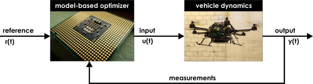
MPC is a feedback control algorithm that uses a process model to predict its output. Based on prediction, the controller makes optimizations to adjust input variables of the plant. MPC deals with multiple inputs and outputs, that can interact with each other and respect constraints.
MPC was implemented in industry in the 1980s, started to be used in other areas thanks to the increase of microprocessors’ computational power. This algorithm requires a lot of memory and a fast processor.
Why use predictive control?
In a MIMO (Multiple Input and Multiple Output) system, if were to use conventional controllers, would have to design and implement many parallel controllers. Since inputs relate to each other, would be very difficult to implement and control the plant. One single MPC can replace many PID controllers.
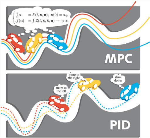
How MPC works?
To predict future output, MPC has a model of plant to make simulations. Need to find which inputs must be applied in the process to get to the reference trajectory. MPC makes many simulations to predict which is the best trajectory to get to reference, in a future time interval and which control inputs must be applied in the process.
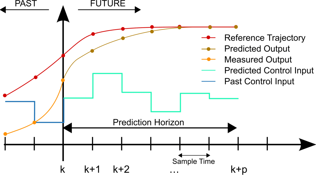
However, MPC can’t make simulations randomly. And then enters the optimizer. The optimization calculation is made to minimize the error between output and reference, with the lowest variation possible in input variables. Because if you vary in excess, you will be too far from reference. Optimization is made with the cost function J. For simplification, this equation has only one control variable. In real situations, there are many variables.
J=\sum_{t=k}^{t=k+p}(W_{e}\cdot e_{k+t}^{2} )+\sum_{t=k}^{t=k+p}(W_{u}\cdot \Delta u_{k+t}^{2})
Where:
- W_{e} and W_{u} are the weighs of error and control variable respectively.
- e_{k+t} is the error (difference between reference and output measure) in an instant of time.
- \Delta u_{k+t} is the variation of control variable.
Trajectory with the lowest cost function is chosen.
Some applications of predictive control
In addition to being used in many industrial processes, other application examples are:
- Robots that need to follow a defined trajectory, need a predictive control to know how to follow this trajectory, respecting constraints to not deviate from it.
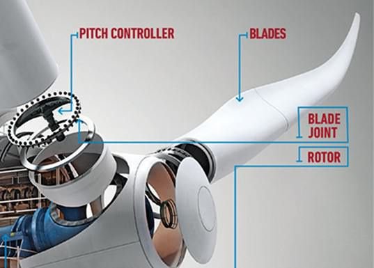
- Wind turbines with pitch controller and speed control, considering fatigue constraints.
- Driverless land vehicles will use predictive control.


